


Generative Adversarial Network
Generative Adversarial Networks (GANs)
What is a GAN?
A Generative Adversarial Network (GAN) is a machine learning setup with two neural networks: a Generator (makes fakes) and a Discriminator (spots fakes). They compete, and both get better over time.
A Generative Adversarial Network (GAN) is a machine learning setup with two neural networks: a Generator (makes fakes) and a Discriminator (spots fakes). They compete, and both get better over time.
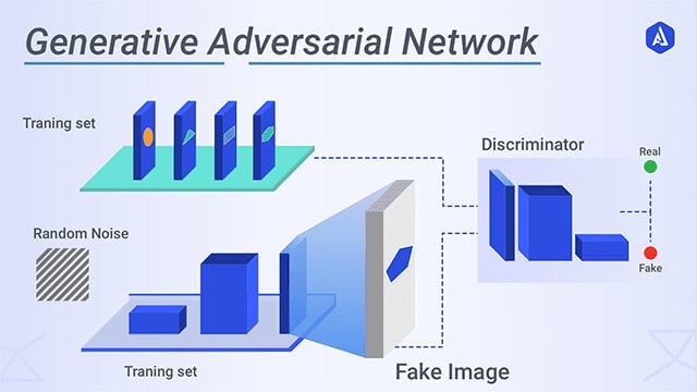
GAN Architecture Explained
| Component | Role | Analogy |
|---|---|---|
| Generator (G) | Creates fake data (like fake images) from random noise. | Forger (makes counterfeits) |
| Discriminator (D) | Tries to tell if data is real (from the dataset) or fake (from the generator). | Detective (spots fakes) |
How it works:
- Generator makes fakes from random noise.
- Discriminator sees both real and fake data, and tries to guess which is which.
- Both networks learn and improve by competing with each other.
The Math Behind GANs (Simple Version)
The GAN Game:
$$ \min_G \max_D V(D, G) = \mathbb{E}_{x \sim p_{data}(x)} [\log D(x)] + \mathbb{E}_{z \sim p_z(z)} [\log(1 - D(G(z)))] $$
$$ \min_G \max_D V(D, G) = \mathbb{E}_{x \sim p_{data}(x)} [\log D(x)] + \mathbb{E}_{z \sim p_z(z)} [\log(1 - D(G(z)))] $$
- $x$: Real data from the dataset
- $z$: Random noise input
- $G(z)$: Fake data made by the generator
- $D(x)$: Probability that $x$ is real
- $D(G(z))$: Probability that the fake is real
What does this mean?
- The discriminator tries to say "real" for real data and "fake" for fakes.
- The generator tries to make fakes so good that the discriminator thinks they're real.
Why Does This Work?
- At first, the generator makes poor fakes, and the discriminator easily spots them.
- Over time, the generator learns to make better fakes, and the discriminator gets pickier.
- Eventually, the generator's fakes are so good that the discriminator can't tell real from fake (it guesses 50/50).
Fun Fact: When GANs are trained well, even humans can have trouble telling the fakes from the real data!
Mathematical Proof: Why GANs Work
1. The Optimal Discriminator
For a fixed generator $G$, the best possible discriminator $D^*$ is:
$$ D^*(x) = \frac{p_{data}(x)}{p_{data}(x) + p_g(x)} $$
where $p_{data}(x)$ is the real data distribution and $p_g(x)$ is the generator's distribution.
For a fixed generator $G$, the best possible discriminator $D^*$ is:
$$ D^*(x) = \frac{p_{data}(x)}{p_{data}(x) + p_g(x)} $$
where $p_{data}(x)$ is the real data distribution and $p_g(x)$ is the generator's distribution.
1. Proof of the Optimal Discriminator
Given a fixed generator $G$, the GAN value function is: $$ V(D, G) = \mathbb{E}_{x \sim p_{\text{data}}}[\log D(x)] + \mathbb{E}_{z \sim p_z}[\log(1 - D(G(z)))] $$ Let $p_g$ be the distribution of $G(z)$. Then: $$ V(D, G) = \int_x p_{\text{data}}(x) \log D(x) dx + \int_x p_g(x) \log(1 - D(x)) dx $$ We maximize $V(D, G)$ with respect to $D(x)$ for each $x$. Define: $$ f(D(x)) = p_{\text{data}}(x) \log D(x) + p_g(x) \log(1 - D(x)) $$ Take the derivative with respect to $D(x)$ and set to zero: $$ \frac{d}{dD(x)} f(D(x)) = \frac{p_{\text{data}}(x)}{D(x)} - \frac{p_g(x)}{1 - D(x)} = 0 $$ Solve for $D(x)$: $$ \frac{p_{\text{data}}(x)}{D(x)} = \frac{p_g(x)}{1 - D(x)} $$ $$ p_{\text{data}}(x)(1 - D(x)) = p_g(x) D(x) $$ $$ p_{\text{data}}(x) = D(x)(p_{\text{data}}(x) + p_g(x)) $$ $$ D^*(x) = \frac{p_{\text{data}}(x)}{p_{\text{data}}(x) + p_g(x)} $$ So, the optimal discriminator is: $$ \boxed{ D^*(x) = \frac{p_{\text{data}}(x)}{p_{\text{data}}(x) + p_g(x)} } $$
Given a fixed generator $G$, the GAN value function is: $$ V(D, G) = \mathbb{E}_{x \sim p_{\text{data}}}[\log D(x)] + \mathbb{E}_{z \sim p_z}[\log(1 - D(G(z)))] $$ Let $p_g$ be the distribution of $G(z)$. Then: $$ V(D, G) = \int_x p_{\text{data}}(x) \log D(x) dx + \int_x p_g(x) \log(1 - D(x)) dx $$ We maximize $V(D, G)$ with respect to $D(x)$ for each $x$. Define: $$ f(D(x)) = p_{\text{data}}(x) \log D(x) + p_g(x) \log(1 - D(x)) $$ Take the derivative with respect to $D(x)$ and set to zero: $$ \frac{d}{dD(x)} f(D(x)) = \frac{p_{\text{data}}(x)}{D(x)} - \frac{p_g(x)}{1 - D(x)} = 0 $$ Solve for $D(x)$: $$ \frac{p_{\text{data}}(x)}{D(x)} = \frac{p_g(x)}{1 - D(x)} $$ $$ p_{\text{data}}(x)(1 - D(x)) = p_g(x) D(x) $$ $$ p_{\text{data}}(x) = D(x)(p_{\text{data}}(x) + p_g(x)) $$ $$ D^*(x) = \frac{p_{\text{data}}(x)}{p_{\text{data}}(x) + p_g(x)} $$ So, the optimal discriminator is: $$ \boxed{ D^*(x) = \frac{p_{\text{data}}(x)}{p_{\text{data}}(x) + p_g(x)} } $$
2. The Value Function at the Optimum
Plugging $D^*(x)$ back into the GAN objective, we get:
$$ V(G, D^*) = \mathbb{E}_{x \sim p_{data}} \left[ \log \frac{p_{data}(x)}{p_{data}(x) + p_g(x)} \right] + \mathbb{E}_{x \sim p_g} \left[ \log \frac{p_g(x)}{p_{data}(x) + p_g(x)} \right] $$
This can be shown to be equal to:
$$ -\log(4) + 2 \cdot \text{JSD}(p_{data} \| p_g) $$ where JSD is the Jensen-Shannon divergence, a way of measuring how different two distributions are.
2. Proof of the Value Function at the Optimum
Plug $D^*(x)$ into the value function: $$ V(G, D^*) = \mathbb{E}_{x \sim p_{\text{data}}}[\log D^*(x)] + \mathbb{E}_{x \sim p_g}[\log(1 - D^*(x))] $$ Recall: - $D^*(x) = \frac{p_{\text{data}}(x)}{p_{\text{data}}(x) + p_g(x)}$ - $1 - D^*(x) = \frac{p_g(x)}{p_{\text{data}}(x) + p_g(x)}$ So, $$ V(G, D^*) = \int_x p_{\text{data}}(x) \log \frac{p_{\text{data}}(x)}{p_{\text{data}}(x) + p_g(x)} dx + \int_x p_g(x) \log \frac{p_g(x)}{p_{\text{data}}(x) + p_g(x)} dx $$ Let $m(x) = \frac{1}{2}(p_{\text{data}}(x) + p_g(x))$. The Jensen-Shannon divergence is: $$ \mathrm{JSD}(p_{\text{data}} \| p_g) = \frac{1}{2} \int_x p_{\text{data}}(x) \log \frac{p_{\text{data}}(x)}{m(x)} dx + \frac{1}{2} \int_x p_g(x) \log \frac{p_g(x)}{m(x)} dx $$ Notice that: $$ \log \frac{p_{\text{data}}(x)}{p_{\text{data}}(x) + p_g(x)} = \log \frac{p_{\text{data}}(x)}{2 m(x)} = \log \frac{p_{\text{data}}(x)}{m(x)} - \log 2 $$ (similar for $p_g(x)$). Therefore, $$ V(G, D^*) = 2 \cdot \mathrm{JSD}(p_{\text{data}} \| p_g) - 2 \log 2 $$ or, $$ V(G, D^*) = -\log 4 + 2 \cdot \mathrm{JSD}(p_{\text{data}} \| p_g) $$ So, at the optimum, the GAN objective is minimized when the generator's distribution matches the real data, and the minimum value is achieved when the Jensen-Shannon divergence is zero.
Plug $D^*(x)$ into the value function: $$ V(G, D^*) = \mathbb{E}_{x \sim p_{\text{data}}}[\log D^*(x)] + \mathbb{E}_{x \sim p_g}[\log(1 - D^*(x))] $$ Recall: - $D^*(x) = \frac{p_{\text{data}}(x)}{p_{\text{data}}(x) + p_g(x)}$ - $1 - D^*(x) = \frac{p_g(x)}{p_{\text{data}}(x) + p_g(x)}$ So, $$ V(G, D^*) = \int_x p_{\text{data}}(x) \log \frac{p_{\text{data}}(x)}{p_{\text{data}}(x) + p_g(x)} dx + \int_x p_g(x) \log \frac{p_g(x)}{p_{\text{data}}(x) + p_g(x)} dx $$ Let $m(x) = \frac{1}{2}(p_{\text{data}}(x) + p_g(x))$. The Jensen-Shannon divergence is: $$ \mathrm{JSD}(p_{\text{data}} \| p_g) = \frac{1}{2} \int_x p_{\text{data}}(x) \log \frac{p_{\text{data}}(x)}{m(x)} dx + \frac{1}{2} \int_x p_g(x) \log \frac{p_g(x)}{m(x)} dx $$ Notice that: $$ \log \frac{p_{\text{data}}(x)}{p_{\text{data}}(x) + p_g(x)} = \log \frac{p_{\text{data}}(x)}{2 m(x)} = \log \frac{p_{\text{data}}(x)}{m(x)} - \log 2 $$ (similar for $p_g(x)$). Therefore, $$ V(G, D^*) = 2 \cdot \mathrm{JSD}(p_{\text{data}} \| p_g) - 2 \log 2 $$ or, $$ V(G, D^*) = -\log 4 + 2 \cdot \mathrm{JSD}(p_{\text{data}} \| p_g) $$ So, at the optimum, the GAN objective is minimized when the generator's distribution matches the real data, and the minimum value is achieved when the Jensen-Shannon divergence is zero.
Conclusion:
- The generator gets better by making $p_g$ (the fake data) as close as possible to $p_{data}$ (the real data).
- When $p_g = p_{data}$, the discriminator can't tell the difference and always outputs 0.5.
- This is what it means for the GAN to "work" – the generator has learned to make perfect fakes!
References
-
Goodfellow, I., Pouget-Abadie, J., Mirza, M., Xu, B., Warde-Farley, D., Ozair, S., Courville, A., & Bengio, Y. (2014). Generative Adversarial Nets. NeurIPS.
- Ian Goodfellow's NIPS 2016 Tutorial: arXiv:1701.00160
- Radford, A., Metz, L., & Chintala, S. (2015). Unsupervised Representation Learning with Deep Convolutional GANs. arXiv:1511.06434.