Graph Neural Networks: From Mathematical Foundations to Recommender Systems
Graph Neural Networks
Graph Neural Networks (GNNs) are a class of deep learning models designed to work with graph-structured data. Unlike traditional neural networks that operate on Euclidean data (images, text), GNNs can capture complex relationships and dependencies in non-Euclidean graph structures. They enable machine learning on networks like social graphs, molecular structures, knowledge graphs, and recommendation systems.
Why Graphs Matter: Beyond Traditional Data Structures
Traditional machine learning models assume that data points are independent and identically distributed (i.i.d.). However, many real-world datasets exhibit complex relational structures:
- Social Networks: Users influence each other's behavior
- Molecular Chemistry: Atom interactions determine properties
- Recommender Systems: User-item interactions reveal preferences
- Knowledge Graphs: Entities are interconnected through relationships
The key insight: Relationships between data points often contain as much information as the data points themselves!
| Data Type | Structure | Traditional ML | Graph-based ML | Key Advantage |
|---|---|---|---|---|
| Images | Grid (2D Euclidean) | CNN | Vision GNN | Captures long-range dependencies |
| Text | Sequence (1D) | RNN/Transformer | Text GNN | Models syntactic relationships |
| Social Networks | Graph (Non-Euclidean) | Feature engineering | GNN | Natural representation |
| Molecules | Graph (Non-Euclidean) | Hand-crafted descriptors | GNN | End-to-end learning |
Mathematical Foundations: Graph Theory Essentials
A graph $G = (V, E)$ consists of:
- Vertices (Nodes): $V = \{v_1, v_2, ..., v_n\}$ - the entities
- Edges: $E \subseteq V \times V$ - the relationships
Types of Graphs:
- Undirected: $(u, v) \in E \Leftrightarrow (v, u) \in E$
- Directed: $(u, v) \in E \not\Rightarrow (v, u) \in E$
- Weighted: Each edge $(u, v)$ has weight $w(u, v)$
The Adjacency Matrix: Encoding Graph Structure
For a graph $G = (V, E)$ with $n$ vertices, the adjacency matrix $A \in \mathbb{R}^{n \times n}$ is defined as: $$A_{ij} = \begin{cases} 1 & \text{if } (v_i, v_j) \in E \\ 0 & \text{otherwise} \end{cases}$$
For weighted graphs: $A_{ij} = w(v_i, v_j)$ if edge exists, 0 otherwise.
Properties:
- Undirected graphs: $A = A^T$ (symmetric)
- Self-loops: $A_{ii} = 1$ if node has self-connection
- Sparsity: Most real graphs are sparse ($|E| \ll n^2$)
The Degree Matrix: Understanding Node Connectivity
The degree of a node $v_i$ is: $d_i = \sum_{j=1}^n A_{ij}$
The degree matrix $D \in \mathbb{R}^{n \times n}$ is a diagonal matrix: $$D_{ij} = \begin{cases} d_i & \text{if } i = j \\ 0 & \text{otherwise} \end{cases}$$
Why degrees matter:
- Centrality: High-degree nodes are often important
- Normalization: Prevents high-degree nodes from dominating
- Random walks: Degree affects transition probabilities
The graph Laplacian combines adjacency and degree information: $$L = D - A$$
Normalized Laplacian: $L_{norm} = D^{-1/2}LD^{-1/2} = I - D^{-1/2}AD^{-1/2}$
Key properties:
- Positive semi-definite: $x^TLx \geq 0$ for all $x$
- Eigenvalues encode graph structure and connectivity
- Used in spectral graph theory and clustering
Graph Convolutional Networks (GCNs): The Foundation
Graph Convolutional Networks extend the concept of convolution to graphs. Instead of convolving over a regular grid (like images), GCNs aggregate information from a node's neighborhood in the graph structure.
Key Insight: A node's representation should be influenced by its neighbors' features, weighted by the strength of their connections.
How GCNs Work: An Intuitive Analogy
Imagine a GCN as a kind of digital gossip network. To figure out who you are (your node embedding), it doesn't just look at your own features; it asks your friends (your neighbors).
- Gather: Each friend tells you about themselves.
- Combine: You aggregate all that information from your friends.
- Transform: You then combine this aggregated info with your own features and pass it through a neural network layer to create a new, updated version of yourself.
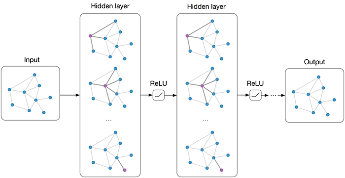
This process is repeated over several layers. So, after one layer, you know about your friends. After two layers, you know about your friends' friends, and so on. This allows the model to learn about the broader graph structure and context.
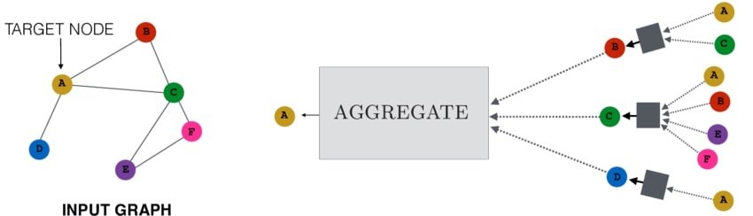
Image 1: Illustrates how GNNs aggregate information from neighboring nodes over multiple layers to create a comprehensive node representation.
GCNs are like CNNs (but for Graphs!)
To better understand the core idea of GCNs, it's helpful to compare them to Convolutional Neural Networks (CNNs), which are widely used for image processing.
- CNNs for Images: A CNN filter slides over a grid of pixels. It computes a new value for a central pixel by performing a weighted average of its immediate neighbors in the grid. This process extracts local features like edges and textures.
- GCNs for Graphs: A GCN operation does something similar, but for a graph. Instead of a fixed grid, the "neighborhood" is defined by the graph's connections. It computes a new feature vector for a node by performing a weighted average of its neighbors' feature vectors. This aggregates information from a node's local network.
This analogy helps bridge the gap between two powerful concepts in deep learning and highlights the core principle of local information aggregation that they share.
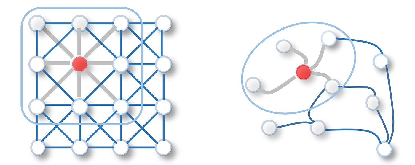
Image 2: Visual comparison of convolution operations in CNNs (on grid-like data) and GCNs (on graph-structured data), highlighting their shared mechanism of local aggregation.
For layer $l$, the forward pass is: $$H^{(l+1)} = \sigma\left(\tilde{A}H^{(l)}W^{(l)}\right)$$ Where:
- $H^{(l)} \in \mathbb{R}^{n \times d_l}$ - node features at layer $l$
- $W^{(l)} \in \mathbb{R}^{d_l \times d_{l+1}}$ - learnable weight matrix
- $\tilde{A}$ - normalized adjacency matrix
- $\sigma$ - activation function (ReLU, etc.)
A complete GCN with $L$ layers:
$H^{(0)} = X$ (input node features)
$H^{(l+1)} = \sigma\left(\tilde{A}H^{(l)}W^{(l)}\right)$ for $l = 0, 1, ..., L-2$
$Z = \text{softmax}\left(\tilde{A}H^{(L-1)}W^{(L-1)}\right)$ (output layer)
Key Properties:
- Localized: Each layer only looks at immediate neighbors
- Scalable: Linear in number of edges $O(|E|)$
- Permutation invariant: Node ordering doesn't matter
GCN Example: Node Classification
Bipartite Graphs: A Special Structure
A bipartite graph $G = (U \cup V, E)$ has two disjoint sets of vertices $U$ and $V$ such that every edge connects a vertex in $U$ to a vertex in $V$. No edges exist within $U$ or within $V$.
Common Examples:
- User-Item graphs: Users connect to items they purchased/rated
- Author-Paper graphs: Authors connect to papers they wrote
- Actor-Movie graphs: Actors connect to movies they appeared in
- Gene-Disease graphs: Genes connect to diseases they influence
Adjacency Matrix for Bipartite Graphs
For a bipartite graph $G = (U \cup V, E)$ with $|U| = m$ and $|V| = n$, we have two representations:
1. Biadjacency Matrix $B \in \mathbb{R}^{m \times n}$: $B_{ij} = \begin{cases} 1 & \text{if } (u_i, v_j) \in E \\ 0 & \text{otherwise} \end{cases}$
2. Full Adjacency Matrix $A \in \mathbb{R}^{(m+n) \times (m+n)}$: $A = \begin{pmatrix} 0_{m \times m} & B \\ B^T & 0_{n \times n} \end{pmatrix}$
GCNs for Bipartite Graphs
For bipartite graphs, we can adapt GCNs to handle two types of nodes:
User node updates: $H_u^{(l+1)} = \sigma\left(B \cdot H_v^{(l)} \cdot W_u^{(l)}\right)$
Item node updates: $H_v^{(l+1)} = \sigma\left(B^T \cdot H_u^{(l)} \cdot W_v^{(l)}\right)$
Where:
- $H_u^{(l)}$ - user embeddings at layer $l$
- $H_v^{(l)}$ - item embeddings at layer $l$
- $W_u^{(l)}, W_v^{(l)}$ - type-specific weight matrices
- $B$ - biadjacency matrix
In bipartite GCNs, user and item representations are updated alternately:
- User update: Aggregate from connected items
- Item update: Aggregate from connected users
- No direct: User-user or item-item connections
This creates a natural collaborative filtering mechanism where users influence items they interact with, and vice versa.
Recommender Systems with Bipartite GNNs
Given a set of users $U$ and items $V$, with observed interactions $R \subset U \times V$, predict which unobserved user-item pairs $(u, v) \notin R$ are likely to result in positive interactions.
Traditional approaches: Matrix factorization, collaborative filtering
GNN advantage: Captures higher-order collaborative signals through multi-hop neighbors
LightGCN removes feature transformation and nonlinear activation:
User embeddings: $\mathbf{e}_u^{(k+1)} = \sum_{i \in N_u} \frac{1}{\sqrt{|N_u|}\sqrt{|N_i|}} \mathbf{e}_i^{(k)}$
Item embeddings: $\mathbf{e}_i^{(k+1)} = \sum_{u \in N_i} \frac{1}{\sqrt{|N_i|}\sqrt{|N_u|}} \mathbf{e}_u^{(k)}$
Final representation: $\mathbf{e}_u = \sum_{k=0}^K \alpha_k \mathbf{e}_u^{(k)}, \quad \mathbf{e}_i = \sum_{k=0}^K \alpha_k \mathbf{e}_i^{(k)}$
Complete Recommender System Example
Advanced Bipartite GNN Architectures
| Model | Key Innovation | Advantages | Use Cases |
|---|---|---|---|
| NGCF | Higher-order connectivity + feature transformation | Captures complex user-item relationships | General recommendation |
| LightGCN | Removes transformations and activations | Simple, efficient, strong performance | Collaborative filtering |
| UltraGCN | Skips message passing entirely | Ultra-fast training and inference | Large-scale systems |
| DGCF | Disentangled representations | Interpretable factors | Explainable recommendations |
Training Bipartite GNNs: Loss Functions and Optimization
For implicit feedback data, BPR optimizes pairwise ranking: $\mathcal{L}_{BPR} = \sum_{(u,i,j) \in D_s} -\ln \sigma(\hat{y}_{ui} - \hat{y}_{uj}) + \lambda ||\Theta||^2$
Where:
- $(u,i,j)$: user $u$, positive item $i$, negative item $j$
- $\hat{y}_{ui} = \mathbf{e}_u^T \mathbf{e}_i$: predicted score
- $\sigma$: sigmoid function
- $\lambda$: L2 regularization coefficient
- $\Theta$: all model parameters
Since we only observe positive interactions, we need to sample negative examples:
- Uniform sampling: Random unobserved items
- Popularity-based: Sample based on item popularity
- Hard negative mining: Focus on challenging negatives
- Dynamic sampling: Adapt sampling during training
Challenge: Unobserved ≠ Negative (users might like items they haven't interacted with yet)
Evaluation Metrics for Recommendation
Recall@K: $Recall@K = \frac{|I_u^{test} \cap I_u^{rec}(K)|}{|I_u^{test}|}$
NDCG@K: $NDCG@K = \frac{DCG@K}{IDCG@K}$
Where $DCG@K = \sum_{i=1}^K \frac{rel_i}{\log_2(i+1)}$
Hit Ratio@K: $HR@K = \frac{\text{# users with at least 1 hit in top-K}}{|\text{test users}|}$
Challenges and Future Directions
- Cold Start: New users/items with no interactions
- Scalability: Large graphs with millions of nodes
- Dynamic Graphs: Interactions change over time
- Fairness: Avoiding bias in recommendations
- Explainability: Understanding why items are recommended
- Privacy: Protecting user interaction data
Implementation Considerations
- Graph preprocessing: Remove very sparse users/items
- Embedding initialization: Use Xavier/He initialization
- Learning rates: Often need different rates for users vs items
- Batch sampling: Sample subgraphs for mini-batch training
- Early stopping: Monitor validation metrics carefully
- Hyperparameter tuning: Layer depth, embedding size, regularization
Conclusion: The Power of Graph Structure in Recommendations
Graph Neural Networks, particularly when applied to bipartite graphs, represent a paradigm shift in how we approach recommendation systems. By naturally modeling the user-item interaction structure as a graph, GNNs can capture complex collaborative filtering signals that traditional matrix factorization methods miss.
The mathematical elegance of bipartite GNNs lies in their ability to propagate information through the graph structure, allowing users to discover items through multi-hop collaborative signals. This approach has proven highly effective in practice, with models like LightGCN achieving state-of-the-art performance while maintaining simplicity and interpretability.
As the field continues to evolve, we can expect further innovations in handling dynamic graphs, improving fairness, and scaling to even larger datasets. The foundation provided by GNNs on bipartite graphs will undoubtedly continue to drive advances in recommender systems and beyond.
References
- Kipf, T. N., & Welling, M. (2016). Semi-supervised classification with graph convolutional networks. arXiv preprint arXiv:1609.02907.
- He, X., Deng, K., Wang, X., Li, Y., Zhang, Y., & Wang, M. (2020). LightGCN: Simplifying and powering graph convolution network for recommendation. SIGIR 2020.
- Wang, X., He, X., Wang, M., Feng, F., & Chua, T. S. (2019). Neural graph collaborative filtering. SIGIR 2019.
- Rendle, S., Freudenthaler, C., Gantner, Z., & Schmidt-Thieme, L. (2009). BPR: Bayesian personalized ranking from implicit feedback. UAI 2009.